None

Multi-view KMeans

from mvlearn.datasets import load_UCImultifeature
from mvlearn.cluster import MultiviewKMeans
from sklearn.cluster import KMeans
import numpy as np
from sklearn.manifold import TSNE
from sklearn.metrics import normalized_mutual_info_score as nmi_score
import matplotlib.pyplot as plt
%matplotlib inline
import warnings
warnings.filterwarnings("ignore")
RANDOM_SEED=5

Load in UCI digits multiple feature data set as an example

# Load dataset along with labels for digits 0 through 4
n_class = 5
data, labels = load_UCImultifeature(select_labeled = list(range(n_class)))

# Just get the first two views of data
m_data = data[:2]

# Helper function to display data and the results of clustering
def display_plots(pre_title, data, labels):

    # plot the views
    plt.figure()
    fig, ax = plt.subplots(1,2, figsize=(14,5))
    dot_size=10
    ax[0].scatter(data[0][:, 0], data[0][:, 1],c=labels,s=dot_size)
    ax[0].set_title(pre_title + ' View 1')
    ax[0].axes.get_xaxis().set_visible(False)
    ax[0].axes.get_yaxis().set_visible(False)

    ax[1].scatter(data[1][:, 0], data[1][:, 1],c=labels,s=dot_size)
    ax[1].set_title(pre_title + ' View 2')
    ax[1].axes.get_xaxis().set_visible(False)
    ax[1].axes.get_yaxis().set_visible(False)

    plt.show()

Single-view and multi-view clustering of the data with 2 views

Here we will compare the performance of the Multi-view and Single-view versions of kmeans clustering. We will evaluate the purity of the resulting clusters from each algorithm with respect to the class labels using the normalized mutual information metric.

As we can see, Multi-view clustering produces clusters with higher purity compared to those produced by clustering on just a single view or by clustering the two views concatenated together.

#################Single-view kmeans clustering#####################
# Cluster each view separately
s_kmeans = KMeans(n_clusters=n_class, random_state=RANDOM_SEED)
s_clusters_v1 = s_kmeans.fit_predict(m_data[0])
s_clusters_v2 = s_kmeans.fit_predict(m_data[1])

# Concatenate the multiple views into a single view
s_data = np.hstack(m_data)
s_clusters = s_kmeans.fit_predict(s_data)

# Compute nmi between true class labels and single-view cluster labels
s_nmi_v1 = nmi_score(labels, s_clusters_v1)
s_nmi_v2 = nmi_score(labels, s_clusters_v2)
s_nmi = nmi_score(labels, s_clusters)
print('Single-view View 1 NMI Score: {0:.3f}\n'.format(s_nmi_v1))
print('Single-view View 2 NMI Score: {0:.3f}\n'.format(s_nmi_v2))
print('Single-view Concatenated NMI Score: {0:.3f}\n'.format(s_nmi))

#################Multi-view kmeans clustering######################

# Use the MultiviewKMeans instance to cluster the data
m_kmeans = MultiviewKMeans(n_clusters=n_class, random_state=RANDOM_SEED)
m_clusters = m_kmeans.fit_predict(m_data)

# Compute nmi between true class labels and multi-view cluster labels
m_nmi = nmi_score(labels, m_clusters)
print('Multi-view NMI Score: {0:.3f}\n'.format(m_nmi))

Single-view View 1 NMI Score: 0.635

Single-view View 2 NMI Score: 0.746

Single-view Concatenated NMI Score: 0.746

Multi-view NMI Score: 0.770

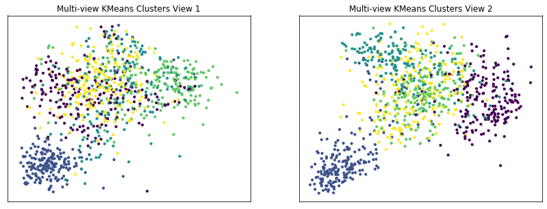
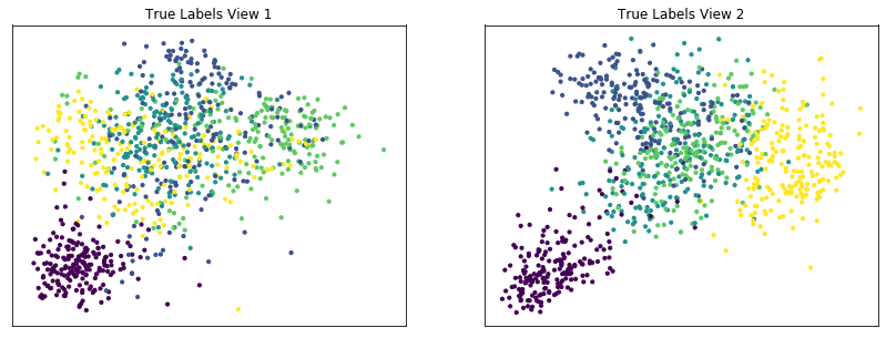
Plot clusters produced by multi-view spectral clustering and the true clusters

We will display the clustering results of the Multi-view kmeans clustering algorithm below, along with the true class labels.

# Running TSNE to display clustering results via low dimensional embedding
tsne = TSNE()
new_data_1 = tsne.fit_transform(m_data[0])
new_data_2 = tsne.fit_transform(m_data[1])

display_plots('Multi-view KMeans Clusters', m_data, m_clusters)
display_plots('True Labels', m_data, labels)

<Figure size 432x288 with 0 Axes>

<Figure size 432x288 with 0 Axes>

Spectral clustering with different parameters

Here we will again compare the performance of the Multi-view and Single-view versions of kmeans clusteringon data with 2 views. We will follow a similar procedure as before, but we will be using a different configuration of parameters for Multi-view Spectral Clustering.

Again, we can see that Multi-view clustering produces clusters with higher purity compared to those produced by clustering on just a single view or by clustering the two views concatenated together.

#################Single-view kmeans clustering#####################
# Cluster each view separately
s_kmeans = KMeans(n_clusters=n_class, random_state=RANDOM_SEED)
s_clusters_v1 = s_kmeans.fit_predict(m_data[0])
s_clusters_v2 = s_kmeans.fit_predict(m_data[1])

# Concatenate the multiple views into a single view
s_data = np.hstack(m_data)
s_clusters = s_kmeans.fit_predict(s_data)

# Compute nmi between true class labels and single-view cluster labels
s_nmi_v1 = nmi_score(labels, s_clusters_v1)
s_nmi_v2 = nmi_score(labels, s_clusters_v2)
s_nmi = nmi_score(labels, s_clusters)
print('Single-view View 1 NMI Score: {0:.3f}\n'.format(s_nmi_v1))
print('Single-view View 2 NMI Score: {0:.3f}\n'.format(s_nmi_v2))
print('Single-view Concatenated NMI Score: {0:.3f}\n'.format(s_nmi))

#################Multi-view kmeans clustering######################

# Use the MultiviewKMeans instance to cluster the data
m_kmeans = MultiviewKMeans(n_clusters=n_class,
        n_init=10, max_iter=6, patience=2, random_state=RANDOM_SEED)
m_clusters = m_kmeans.fit_predict(m_data)

# Compute nmi between true class labels and multi-view cluster labels
m_nmi = nmi_score(labels, m_clusters)
print('Multi-view NMI Score: {0:.3f}\n'.format(m_nmi))

Single-view View 1 NMI Score: 0.635

Single-view View 2 NMI Score: 0.746

Single-view Concatenated NMI Score: 0.746

Multi-view NMI Score: 0.747