None

Deep CCA (DCCA)

In this example, we show how to used Deep CCA to uncover latent correlations between views.

from mvlearn.embed import DCCA

from mvlearn.datasets import GaussianMixture
from mvlearn.plotting import crossviews_plot
import numpy as np
import matplotlib.pyplot as plt
%matplotlib inline

Polynomial-Transformed Latent Correlation

Latent variables are sampled from two multivariate Gaussians with equal prior probability. Then a polynomial transformation is applied and noise is added independently to both the transformed and untransformed latents.

n_samples = 2000
centers = [[0,1], [0,-1]]
covariances = [np.eye(2), np.eye(2)]
GM = GaussianMixture(n_samples, centers, covariances, random_state=42,
                     shuffle=True, shuffle_random_state=42)
GM = GM.sample_views(transform='poly', n_noise=2)

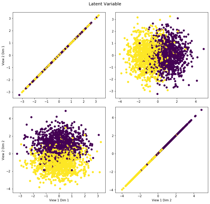
The latent data is plotted against itself to reveal the underlying distribtution.

crossviews_plot([GM.latent, GM.latent], labels=GM.y, title='Latent Variable', equal_axes=True)

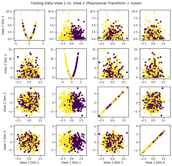
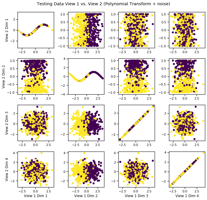
The noisy latent variable (view 1) is plotted against the transformed latent variable (view 2), an example of a dataset with two views.

# Split data into train and test segments
Xs_train = []
Xs_test = []
max_row = int(GM.Xs[0].shape[0] * .7)
Xs, y = GM.get_Xy(latents=False)
for X in Xs:
    Xs_train.append(X[:max_row, :])
    Xs_test.append(X[max_row:, :])
y_train = y[:max_row]
y_test = y[max_row:]

crossviews_plot(Xs_test, labels=y_test, title='Testing Data View 1 vs. View 2 (Polynomial Transform + noise)', equal_axes=True)

Fit DCCA model to uncover latent distribution

The output dimensionality is still 4.

# Define parameters and layers for deep model
features1 = Xs_train[0].shape[1] # Feature sizes
features2 = Xs_train[1].shape[1]
layers1 = [1024, 512, 4] # nodes in each hidden layer and the output size
layers2 = [1024, 512, 4]

dcca = DCCA(input_size1=features1, input_size2=features2, n_components=4,
            layer_sizes1=layers1, layer_sizes2=layers2)
dcca.fit(Xs_train)
Xs_transformed = dcca.transform(Xs_test)

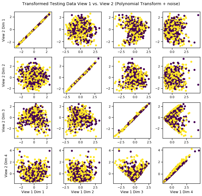
Visualize the transformed data

We can see that it has uncovered the latent correlation between views.

crossviews_plot(Xs_transformed, labels=y_test, title='Transformed Testing Data View 1 vs. View 2 (Polynomial Transform + noise)', equal_axes=True)

Sinusoidal-Transformed Latent Correlation

Following the same procedure as above, latent variables are sampled from two multivariate Gaussians with equal prior probability. This time, a sinusoidal transformation is applied and noise is added independently to both the transformed and untransformed latents.

n = 2000
mu = [[0,1], [0,-1]]
sigma = [np.eye(2), np.eye(2)]
class_probs = [0.5, 0.5]
GM = GaussianMixture(mu,sigma,n,class_probs=class_probs, random_state=42,
                     shuffle=True, shuffle_random_state=42)
GM = GM.sample_views(transform='sin', n_noise=2)

# Split data into train and test segments
Xs_train = []
Xs_test = []
max_row = int(GM.Xs[0].shape[0] * .7)
for X in GM.Xs:
    Xs_train.append(X[:max_row, :])
    Xs_test.append(X[max_row:, :])
y_train = GM.y[:max_row]
y_test = GM.y[max_row:]

crossviews_plot(Xs_test, labels=y_test, title='Testing Data View 1 vs. View 2 (Polynomial Transform + noise)', equal_axes=True)

Fit DCCA model to uncover latent distribution

The output dimensionality is still 4.

# Define parameters and layers for deep model
features1 = Xs_train[0].shape[1] # Feature sizes
features2 = Xs_train[1].shape[1]
layers1 = [1024, 512, 4] # nodes in each hidden layer and the output size
layers2 = [1024, 512, 4]

dcca = DCCA(input_size1=features1, input_size2=features2, n_components=4,
            layer_sizes1=layers1, layer_sizes2=layers2)
dcca.fit(Xs_train)
Xs_transformed = dcca.transform(Xs_test)

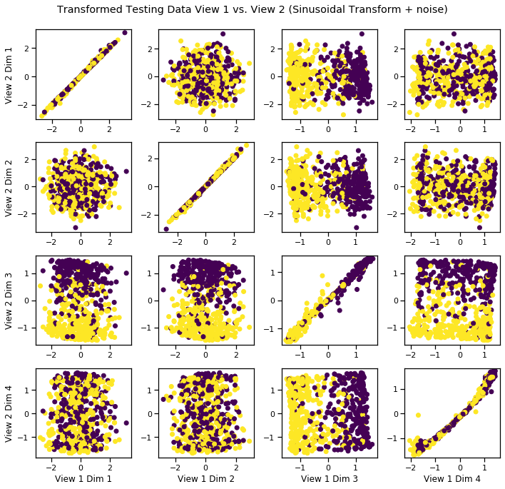
Visualize the transformed data

We can see that it has uncovered the latent correlation between views.

crossviews_plot(Xs_transformed, labels=y_test, title='Transformed Testing Data View 1 vs. View 2 (Sinusoidal Transform + noise)', equal_axes=True)