Assessing the Conditional Independence Views Requirement of Multi-view Spectral Clustering
[2]:
import numpy as np
from numpy.random import multivariate_normal
import scipy as scp
from mvlearn.cluster.mv_spectral import MultiviewSpectralClustering
from sklearn.cluster import SpectralClustering
from sklearn.metrics import normalized_mutual_info_score as nmi_score
from sklearn.datasets import fetch_covtype
import matplotlib.pyplot as plt
%matplotlib inline
from sklearn.manifold import TSNE
import warnings
warnings.filterwarnings("ignore")
RANDOM_SEED=10
Creating an artificial dataset where the conditional independence assumption between views holds
Here, we create an artificial dataset where the conditional independence assumption between views, given the true labels, is enforced. Our artificial dataset is derived from the forest covertypes dataset from the scikit-learn package. This dataset is comprised of 7 different classes, with with 54 different numerical features per sample. To create our artificial data, we will select 500 samples from each of the first 6 classes in the dataset, and from these, construct 3 artificial classes with 2 views each.
[3]:
def get_ci_data(num_samples=500):

    #Load in the vectorized news group data from scikit-learn package
    cov = fetch_covtype()
    all_data = np.array(cov.data)
    all_targets = np.array(cov.target)

    #Set class pairings as described in the multiview clustering paper
    view1_classes = [1, 2, 3]
    view2_classes = [4, 5, 6]

    #Create lists to hold data and labels for each of the classes across 2 different views
    labels =  [num for num in range(len(view1_classes)) for _ in range(num_samples)]
    labels = np.array(labels)
    view1_data = list()
    view2_data = list()

    #Randomly sample items from each of the selected classes in view1
    for class_num in view1_classes:
        class_data = all_data[(all_targets == class_num)]
        indices = np.random.choice(class_data.shape[0], num_samples)
        view1_data.append(class_data[indices])
    view1_data = np.concatenate(view1_data)


    #Randomly sample items from each of the selected classes in view2
    for class_num in view2_classes:
        class_data = all_data[(all_targets == class_num)]
        indices = np.random.choice(class_data.shape[0], num_samples)
        view2_data.append(class_data[indices])
    view2_data = np.concatenate(view2_data)

    #Shuffle and normalize vectors
    shuffled_inds = np.random.permutation(num_samples * len(view1_classes))
    view1_data = np.vstack(view1_data)
    view2_data = np.vstack(view2_data)
    view1_data = view1_data[shuffled_inds]
    view2_data = view2_data[shuffled_inds]
    magnitudes1 = np.linalg.norm(view1_data, axis=0)
    magnitudes2 = np.linalg.norm(view2_data, axis=0)
    magnitudes1[magnitudes1 == 0] = 1
    magnitudes2[magnitudes2 == 0] = 1
    magnitudes1 = magnitudes1.reshape((1, -1))
    magnitudes2 = magnitudes2.reshape((1, -1))
    view1_data /= magnitudes1
    view2_data /= magnitudes2
    labels = labels[shuffled_inds]
    return [view1_data, view2_data], labels
Creating a function to perform both single-view and multi-view spectral clustering
In the following function, we will perform single-view spectral clustering on the two views separately and on them concatenated together. We also perform multi-view clustering using the multi-view algorithm. We will also compare the performance of multi-view and single-view versions of spectral clustering. We will evaluate the purity of the resulting clusters from each algorithm with respect to the class labels using the normalized mutual information metric.
[4]:
def perform_clustering(seed, m_data, labels, n_clusters):

    #################Single-view spectral clustering#####################
    # Cluster each view separately
    s_spectral = SpectralClustering(n_clusters=n_clusters, random_state=RANDOM_SEED, n_init=100)
    s_clusters_v1 = s_spectral.fit_predict(m_data[0])
    s_clusters_v2 = s_spectral.fit_predict(m_data[1])

    # Concatenate the multiple views into a single view
    s_data = np.hstack(m_data)
    s_clusters = s_spectral.fit_predict(s_data)

    # Compute nmi between true class labels and single-view cluster labels
    s_nmi_v1 = nmi_score(labels, s_clusters_v1)
    s_nmi_v2 = nmi_score(labels, s_clusters_v2)
    s_nmi = nmi_score(labels, s_clusters)
    print('Single-view View 1 NMI Score: {0:.3f}\n'.format(s_nmi_v1))
    print('Single-view View 2 NMI Score: {0:.3f}\n'.format(s_nmi_v2))
    print('Single-view Concatenated NMI Score: {0:.3f}\n'.format(s_nmi))

    #################Multi-view spectral clustering######################

    # Use the MultiviewSpectralClustering instance to cluster the data
    m_spectral = MultiviewSpectralClustering(n_clusters=n_clusters, random_state=RANDOM_SEED, n_init=100)
    m_clusters = m_spectral.fit_predict(m_data)

    # Compute nmi between true class labels and multi-view cluster labels
    m_nmi = nmi_score(labels, m_clusters)
    print('Multi-view Concatenated NMI Score: {0:.3f}\n'.format(m_nmi))

    return m_clusters
Creating a function to display data and the results of clustering
The following function plots both views of data given a dataset and corresponding labels.
[5]:
def display_plots(pre_title, data, labels):

    # plot the views
    plt.figure()
    fig, ax = plt.subplots(1,2, figsize=(14,5))
    dot_size=10
    ax[0].scatter(new_data[0][:, 0], new_data[0][:, 1],c=labels,s=dot_size)
    ax[0].set_title(pre_title + ' View 1')
    ax[0].axes.get_xaxis().set_visible(False)
    ax[0].axes.get_yaxis().set_visible(False)

    ax[1].scatter(new_data[1][:, 0], new_data[1][:, 1],c=labels,s=dot_size)
    ax[1].set_title(pre_title + ' View 2')
    ax[1].axes.get_xaxis().set_visible(False)
    ax[1].axes.get_yaxis().set_visible(False)

    plt.show()
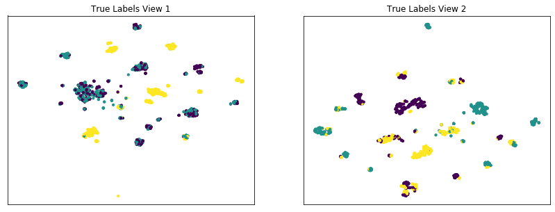
Comparing multi-view and single-view spectral clustering on our data set with conditionally independent views
The co-training framework relies on the fundamental assumption that data views are conditionally independent. If all views are informative and conditionally independent, then Multi-view Spectral Clustering is expected to produce higher quality clusters than Single-view Spectral Clustering, for either view or for both views concatenated together. Here, we will evaluate the quality of clusters by using the normalized mutual information metric, which is essentially a measure of the purity of clusters with respect to the true underlying class labels.
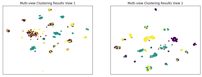
As we see below, Multi-view Spectral Clustering produces clusters with lower purity than those produced by Single-view Spectral clustering on the concatenated views, which is surprising.
[6]:
data, labels = get_ci_data()
m_clusters = perform_clustering(RANDOM_SEED, data, labels, 3)

# Running TSNE to display clustering results via low dimensional embedding
tsne = TSNE()
new_data = list()
new_data.append(tsne.fit_transform(data[0]))
new_data.append(tsne.fit_transform(data[1]))
display_plots('True Labels', new_data, labels)
display_plots('Multi-view Clustering Results', new_data, m_clusters)
Single-view View 1 NMI Score: 0.316

Single-view View 2 NMI Score: 0.500

Single-view Concatenated NMI Score: 0.758

Multi-view Concatenated NMI Score: 0.552
<Figure size 432x288 with 0 Axes>
<Figure size 432x288 with 0 Axes>
Creating an artificial dataset where the conditional independence assumption between views does not hold
Here, we create an artificial dataset where the conditional independence assumption between views, given the true labels, is violated. We again derive our dataset from the forest covertypes dataset from sklearn. However, this time, we use only the first 3 classes of the dataset, which will correspond to the 3 clusters for view 1. To produce view 2, we will apply a simple nonlinear transformation to view 1 using the logistic function, and we will apply a negligible amount of noise to the second view to avoid convergence issues. This will result in a dataset where the correspondance between views is very high.
[7]:
def get_cd_data(num_samples=500):

    #Load in the vectorized news group data from scikit-learn package
    cov = fetch_covtype()
    all_data = np.array(cov.data)
    all_targets = np.array(cov.target)

    #Set class pairings as described in the multiview clustering paper
    view1_classes = [1, 2, 3]
    view2_classes = [4, 5, 6]

    #Create lists to hold data and labels for each of the classes across 2 different views
    labels =  [num for num in range(len(view1_classes)) for _ in range(num_samples)]
    labels = np.array(labels)
    view1_data = list()
    view2_data = list()

    #Randomly sample 500 items from each of the selected classes in view1
    for class_num in view1_classes:
        class_data = all_data[(all_targets == class_num)]
        indices = np.random.choice(class_data.shape[0], num_samples)
        view1_data.append(class_data[indices])
    view1_data = np.concatenate(view1_data)


    #Construct view 2 by applying a nonlinear transformation
    #to data from view 1 comprised of a linear transformation
    #and a logistic nonlinearity
    t_mat =  np.random.random((view1_data.shape[1], 50))
    noise = 0.005 - 0.01*np.random.random((view1_data.shape[1], 50))
    t_mat *= noise
    transformed = view1_data @ t_mat
    view2_data = scp.special.expit(transformed)

    #Shuffle and normalize vectors
    shuffled_inds = np.random.permutation(num_samples * len(view1_classes))
    view1_data = np.vstack(view1_data)
    view2_data = np.vstack(view2_data)
    view1_data = view1_data[shuffled_inds]
    view2_data = view2_data[shuffled_inds]
    magnitudes1 = np.linalg.norm(view1_data, axis=0)
    magnitudes2 = np.linalg.norm(view2_data, axis=0)
    magnitudes1[magnitudes1 == 0] = 1
    magnitudes2[magnitudes2 == 0] = 1
    magnitudes1 = magnitudes1.reshape((1, -1))
    magnitudes2 = magnitudes2.reshape((1, -1))
    view1_data /= magnitudes1
    view2_data /= magnitudes2
    labels = labels[shuffled_inds]
    return [view1_data, view2_data], labels
Comparing multi-view and single-view spectral clustering on our data set with conditionally dependent views
As mentioned before, the co-training framework relies on the fundamental assumption that data views are conditionally independent. Here, we will again compare the performance of single-view and multi-view spectral clustering using the same methods as before, but on our conditionally dependent dataset.
As we see below, Multi-view Spectral Clustering does not beat the best Single-view spectral clustering performance with respect to purity, since that the views are conditionally dependent.
[8]:
data, labels = get_cd_data()
m_clusters = perform_clustering(RANDOM_SEED, data, labels, 3)
Single-view View 1 NMI Score: 0.327

Single-view View 2 NMI Score: 0.160

Single-view Concatenated NMI Score: 0.239

Multi-view Concatenated NMI Score: 0.308